Merklizing the key/value store for fun and profit
Joel Gustafson / Posts / 2023-05-04
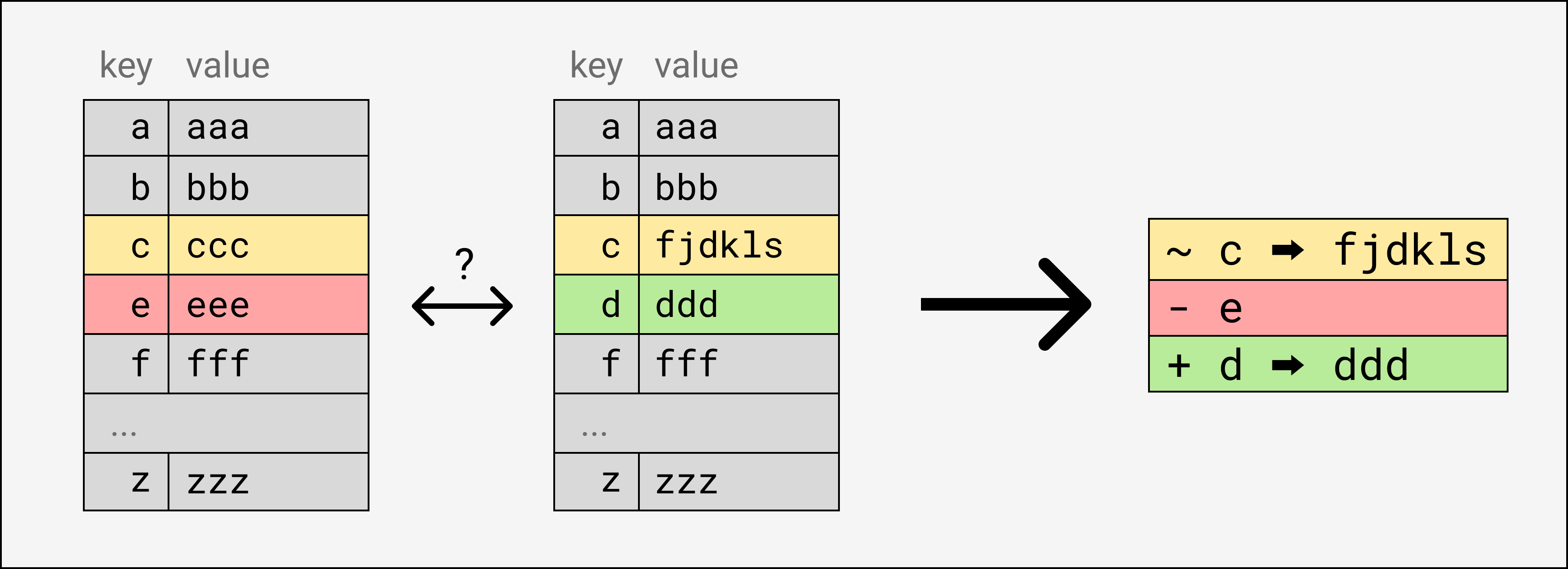
Suppose you and I each have a local key/value store. We suspect our key/value stores have mostly the same contents, but that there might be a few differences: a couple entries that you have that I don’t, that I have that you don’t, or conflicting values for the same key. What’s the best way for us to compare the content of our databases and identify the differences?
Naively, I could send you all of my entries, and you can send me all of your entries. Or I could send you all of my entries, and you could iterate over them and just send me back the diff. But this is still linear in the number of entries.
If you and I care enough about making diffs efficient, we can both maintain a special kind of merkle tree called a Prolly Tree that allows us to skip large sections of shared entries and identify conflicts in logarithmic time. This “merkle syncing” capability is a powerful and versatile peer-to-peer primitive and can be used as a natural persistence layer for CRDT systems, an “rsync for key/value stores”, the foundation of a mutable multi-writer decentralized database, and much more.
Prolly Trees and their cousin Merkle Search Trees are new ideas but are already used by ATProto / BlueSky, Dolt, and others. There are some key differences that make the approach here particularly easy to implement as a wrapper around existing key/value stores.
We'll give a short overview of merkle trees in general, walk through the design of a merklized key/value store, see some example applications, introduce two reference implementations, and wrap up with a comparison to other projects.
#Table of Contents
#Background
If you’re already a merkle tree guru and the prospect of using them to efficiently diff key/value stores seems natural to you, feel free to skip this section.
Merkle trees are simpler than they sound. It just describes a tree whose nodes have been labelled with hashes. The leaves have the hash of their “value” (whatever that means for that particular tree), and every parent node has the hash of the hashes of its children. This means merkle trees have to be built from the leaves up, since the hashes at each layer depend on the hashes of the layer below.
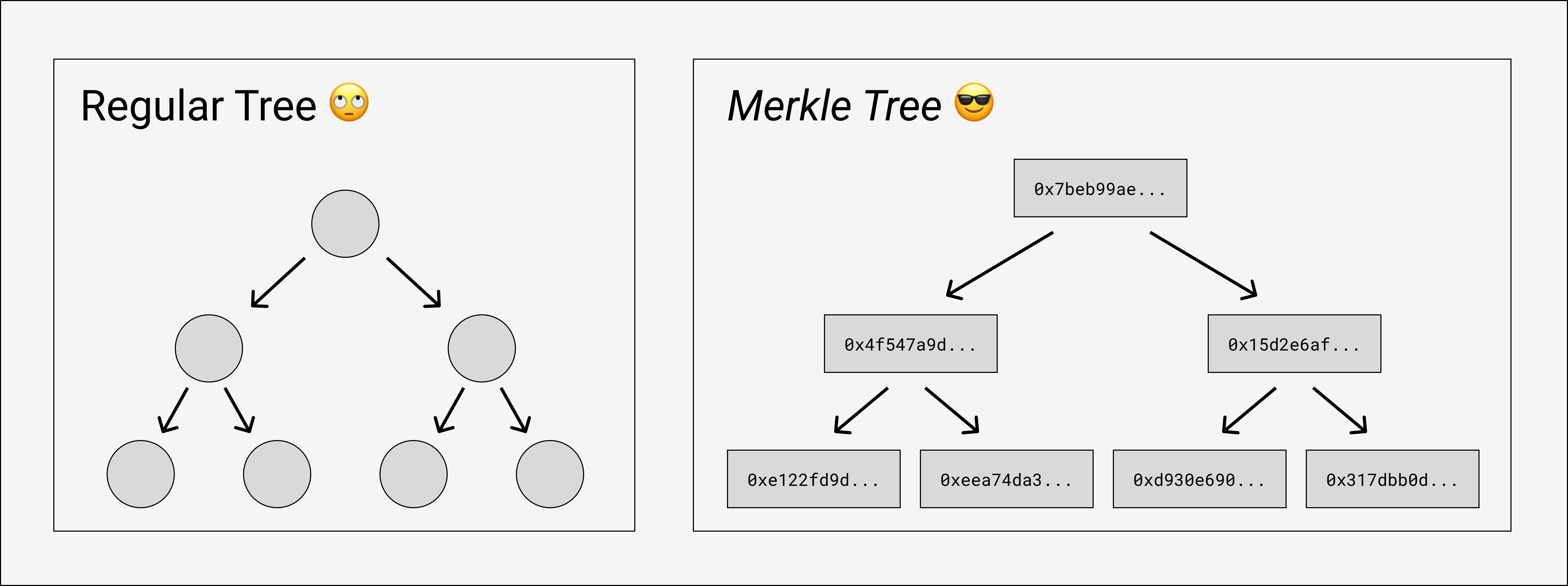
That’s it! Merklizing a tree is just adding these recursive node hashes and keeping them up-to-date when the leaves change.
The goal of merklizing things is usually related to the fact that the root hash uniquely identifies the entire tree - if any of the values of the leaves were to change, the leaf’s hash would change, which would make its parent’s hash change, and so on, all the way up to the root. If two merkle trees have the same root hash, you know for sure they have the values all throughout the tree.
Let’s look at two prominent applications of merkle trees: content-addressed filesystems and commitment schemes.
#Filesystems
IPFS uses merkle trees to represent files and directories. An IPFS identifier is the hash of a PBNode Protobuf struct, shown below.
message PBLink {
  optional bytes Hash = 1;
  optional string Name = 2;
  optional uint64 Tsize = 3;
}

message PBNode {
  repeated PBLink Links = 2;
  optional bytes Data = 1;
}
In the simplest case, files are represented as nodes with the raw file as the Data and no links, and directories are represented as nodes with no Data and a named link for every child file or subdirectory.
Since a directory is identified by the hash of the serialized list of its entries, and each serialized entry has its own hash, we get a system where arbitrarily large directory trees can be uniquely identified with a single constant-size hash. These hashes allow IPFS to be “self-authenticating”: users request content by hash, and can simply hash the returned bytes themselves to ensure they’ve received what they expect.
Another property that we get for free is automatic deduplication. When you ask the IPFS CLI to download a directory, it has to do it step by step, resolving the root node first, and then resolving the links to its child nodes, and then their children, and so on. Internally, IPFS stores merkle nodes by hash in a key/value store in your ~/.ipfs directory, and at every step in that iterative resolution process, it will check the local database first to see if it already has the node it wants. So if you publish two large directories that are mostly the same with just a few differences, like successive versions of a container image, then people who have already downloaded one will only have to download the files that have actually changed, plus the directories in the path to the root.
#Commitment schemes
Another place that merkle trees pop up is in commitment schemes. Suppose you’re a rock star, and you have a list of your close friends that you want to allow backstage at your concerts. You could give the whole list to the security staff, but you’re very popular, and have tons of close friends, any of whom might show up, and security doesn’t want to handle such a big list and do a O(n) table scan every time someone asks to get in.
So instead, you build a binary merkle tree using your friends’ names (or public keys or whatever) as the leaves. Each friend gets hashed, each pair of leaf hashes gets hashed into a level-2 hash, each pair of level-2 hashes gets hashed into a level-3 hash, and so on until there’s just one root hash left. If at any level there’s a lone node left at the end, that’s fine, it just gets hashed by itself.
Now what? You give the root hash to security, and email each of your friends their own unique path of nodes from their leaf up to the root. Each node in the path contains the hash of the previous node in the path and the hash of the previous node’s neighbor, if it exists. When your friends want to get in, they show security their merkle path. Security re-hashes each node in the path, starting at the leaf; checks that it’s one of the hashes included in the next node; and verifies that the path ends with the same root hash that you gave them in advance. Your friends use their merkle paths to prove inclusion in a set uniquely identified by a single constant-size hash, and it only takes O(log(n)) hashes instead of the O(n) table scan.
Why wouldn’t you just give security the whole list and ask them to build an index over it? Why not use a database? One reason might be because security is running entirely on a blockchain like Ethereum (don’t ask me what this means in the analogy) and storing data with them is super expensive. The merkle tree lets you compress the data you need to commit into a constant-size hash. The tradeoff is that your friends have to remember their merkle paths.
#Design
It certainly feels like merkle trees could help us sync our key/value stores. We saw a hint of the basic operating principle in how IPFS automatically deduplicates files; here, our goal is to deduplicate shared subsets of key/value entries.
The only difference is that filesystems already have a tree structure, but the key/value interface is just a logically flat array of entries. This simplicity is part of why they’re are so popular. Even though users often end up rolling their own vaguely hierarchical key format, the flexibility and promise of consistent performance makes them easy to reason about.
To merklize our key/value entries, we’ll have to build up our own tree structure. This doesn’t sound like a problem - after all, this is what we had to do for commitment schemes.
#Fixed-size chunking
Suppose you have a key/value store with entries
key │ value
────┼──────
  a │ foo
  b │ bar
  c │ baz
  d │ qux
... and I have a key/value store with entries
key │ value
────┼──────
  a │ foo
  b │ bar
  c │ eee
  d │ qux
We each build a simple binary merkle tree. To do this, we first need to agree on an encoding e: (key: []byte, value: []byte) => []byte to turn each key/value pair into a leaf value that can be hashed. It’s important to hash both the key and value as part of the leaves, but the specific format doesn’t matter as long as it’s injective and everyone does it the same way.
We sort the entries lexicographically by key, encode the entries to get values for the leaves, and build up a binary tree, labelling each node the hash of its children’s hashes.
┌────┐                            ┌────┐
             │ y0 │                            │ y0'│
             └────┘                            └────┘
                │                                 │
        ┌───────┴───────┐                 ┌───────┴───────┐
        │               │                 │               │
     ┌────┐          ┌────┐            ┌────┐          ┌────┐
     │ x0 │          │ x1 │            │ x0'│          │ x1'│
     └────┘          └────┘            └────┘          └────┘
        │               │                 │               │
   ┌────┴──┐       ┌────┴──┐         ┌────┴──┐       ┌────┴──┐
   │       │       │       │         │       │       │       │
┌─────┐ ┌─────┐ ┌─────┐ ┌─────┐   ┌─────┐ ┌─────┐ ┌─────┐ ┌─────┐
│a:foo│ │b:bar│ │c:baz│ │d:qux│   │a:foo│ │b:bar│ │c:eee│ │d:qux│
└─────┘ └─────┘ └─────┘ └─────┘   └─────┘ └─────┘ └─────┘ └─────┘
You’d get a tree with hashes
x0 = h(e("a", "foo"), e("b", "bar"))x1 = h(e("c", "baz"), e("d", "qux"))y0 = h(x0, x1)
and I would get a tree with hashes
x0' = h(e("a", "foo"), e("b", "bar")) = x0x1' = h(e("c", "eee"), e("d", "qux"))y0' = h(x0', x1')
Remember that our goal is to enumerate the differences. You can probably guess at the approach. We start by exchanging root hashes - if they match, great! We know for sure that we have the exact same trees. If they don’t, then we exchange the hashes of the root’s children. We recurse into subtrees whose hashes don’t match and skip subtrees whose hashes do match.
In the example, we find that y0 != y0', so you send me x0 and x1, and I send you x0' and x1'. We then look at those and find that x0 == x0' but x1 != x1', so you just send me c:baz and d:qux and I send you c:eee and d:qux. It seems complicated, but the process scales logarithmically with the size of the tree, which is pretty nifty. Of course, that’s just if a single entry conflicts. If enough entries conflict, there’s no way around sending the entire tree anyway.
#Offset-sensitivity
Unfortunately, here’s another case where we end up sending the entire tree:
┌────┐
                                                       │ z0'│
                                                       └────┘
                                                          │
                                                  ┌───────┴──────────┐
                                                  │                  │
                                               ┌────┐             ┌────┐
             ┌────┐                            │ y0'│             │ y1'│
             │ y0 │                            └────┘             └────┘
             └────┘                               │                  │
                │                         ┌───────┴──────┐           │
        ┌───────┴───────┐                 │              │           │
        │               │                 │              │           │
     ┌────┐          ┌────┐            ┌────┐         ┌────┐      ┌────┐
     │ x0 │          │ x1 │            │ x0'│         │ x1'│      │ x2'│
     └────┘          └────┘            └────┘         └────┘      └────┘
        │               │                 │              │           │
   ┌────┴──┐       ┌────┴──┐         ┌────┴──┐       ┌───┴───┐       │
   │       │       │       │         │       │       │       │       │
┌─────┐ ┌─────┐ ┌─────┐ ┌─────┐   ┌─────┐ ┌─────┐ ┌─────┐ ┌─────┐ ┌─────┐
│a:foo│ │b:bar│ │c:baz│ │d:qux│   │A:AAA│ │a:foo│ │b:bar│ │c:baz│ │d:qux│
└─────┘ └─────┘ └─────┘ └─────┘   └─────┘ └─────┘ └─────┘ └─────┘ └─────┘
The only difference is that I inserted a new entry A:AAA at the beginning of the tree (capital letters sort before lower-case letters). But because we pair nodes together starting at the beginning, the new entry offsets the entire rest of the tree, giving us no matching hashes at all.
Building binary trees this way is brittle, and the same goes for using fixed-sized chunks of any size. Even though we have lots of common entries, they don’t result in matching higher-level hashes unless they happen to align on chunk boundaries. Plus, it can’t be incrementally maintained. When a new entry gets inserted or an old one gets deleted, you have to throw away the entire tree and re-build it all from the ground up.
This is unfortunate because fixed-size chunking has some otherwise great properties that we want from a tree-building algorithm: it’s simple, it always produces balanced trees, it can be used with any chunk size, and it’s deterministic.
Determinism is critical. Remember, our goal is identify and skip shared subsets of key/value entries by getting them to translate into shared high-level merkle tree nodes, since those can be compared by hash. If the structure of our merkle tree depends on the insertion order of the entries, or is anything other than a pure function of the content of the leaves, then we ruin our chances of recognizing and skipping those shared subsets of entries.
How can we design a merkle tree that’s deterministic but not brittle?
#Content-defined chunking
The brittleness of fixed-size chunking is a problem that appears in file sharing systems too. By default, IPFS splits large files into 262144-byte chunks to enable torrent-style concurrent downloads (this is why the PBNode structs don’t always map one-to-one with files and directories). That means that all of a large file’s chunks change if the file is edited near the beginning. We’re kind of moving the goalposts here, but wouldn’t it be nice if they could deduplicate chunks within two versions of a large file too?
Lucky for us, there are already well-known techniques for mitigating offset-sensitivity within files (IPFS supports several --chunker options). The simplest is to use a rolling hash function to derive content-defined chunk boundaries.
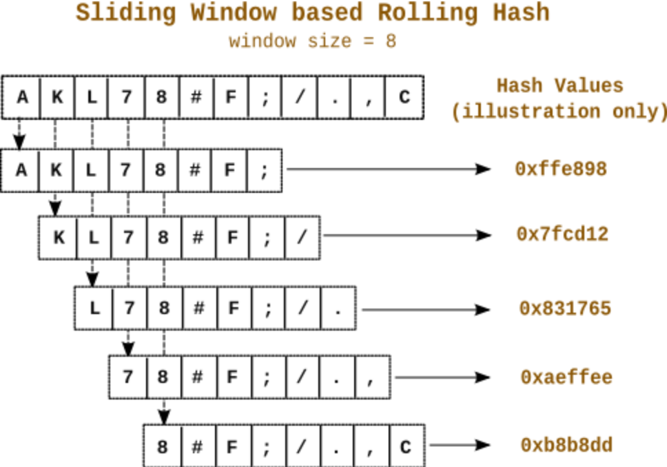
A rolling hash function hashes a moving window of bytes in a stream, effectively hashing just the last n bytes, every byte. You can use a this to chunk a file by starting a new chunk at every byte whose hash begins with a certain number of leading binary zeros. Since the hash is a pure function of window, a stream of bytes will get chunked in the same way regardless of where in the file it appears.
You can set the threshold to a long prefix of zeros to get generally larger chunks, or a short prefix to get generally smaller chunks. In practice, it’s common to add minimum and maximum sizes, or other variations to control the distribution of chunk sizes. This technique even predates the web; rsync (file syncing tool and Dropbox killer) has been doing this since 1996!
(Speaking of rsync, couldn’t we just rsync a database image? Well... yes. rsync lets you do efficient replication from a single-source-of-truth server, and if that’s all you want, you don’t need merkle trees. But you can do much more general things with a merklized key/value store than just replication. We’ll get into this in detail later.)
#Content-defined merkle trees
To apply this idea to our merkle tree, we don’t even need a rolling hash function since we’re not working with byte streams. We can simply use the hashes of the nodes themselves to deterministically divide them into sibling groups, and this will create a tree whose structure is robust to insertions and deletions. For now, we’ll just think about building the tree from scratch and worry about incremental maintenance later.
Let’s say we want the nodes of our merkle tree to have Q children on average. The intuition is to divide up the space of possible hashes into Q evenly-sized buckets, and have the one-in-Q nodes that fall into the first bucket mark boundaries between parents. Here’s the rule:
A node is the first child of its parent if
u32(node.hash[0..4]) < (2^32 / Q).
We call these nodes boundary nodes. A boundary node is the first child of a new parent, and a non-boundary nodes are siblings of the previous boundary node.
That’s it! This totally determines the structure of the tree. You can imagine scanning across a layer, testing each node’s boundary status, creating a new parent on the next level if it’s a boundary node, or adding it as a child of the previous parent if not. Once we finish creating parents for a level, we calculate their hashes by hashing the hashes of all their children in order, and repeat the whole process level after level until there’s just one root node left.
There’s just one more twist: we add a special anchor node at the beginning of every level, which is always the first child of its parent, which is also always an anchor node. This gives a stable backbone to the tree - it will make our lives easier when we get to incremental maintenance, and means that even the empty key/value store has a well-defined root node (the leaf-level anchor node). The leaf-level anchor node’s hash is the hash of the empty input h().
With all this in mind, let’s draw out a larger example tree. The boundary nodes (with hashes below the 2^32/Q threshold) have bold/double borders. Each node is labelled with the key of their first leaf-level entry. This makes it easy to address any node by (level, key), with level = 0 for the leaves and key = null for the anchor nodes. Arranged rectangularly, with first sibling/next sibling arrows instead of parent-child arrows, the whole thing looks more like a skip list than a tree:
╔════╗
 level 4    ║root║
            ╚════╝
              │
              ▼
            ╔════╗                                                               ┌─────┐
 level 3    ║null║ ─────────────────────────────────────────────────────────────▶│  g  │
            ╚════╝                                                               └─────┘
              │                                                                     │
              ▼                                                                     ▼
            ╔════╗                                                               ╔═════╗                                                     ┌─────┐
 level 2    ║null║ ─────────────────────────────────────────────────────────────▶║  g  ║   ─────────────────────────────────────────────────▶│  m  │
            ╚════╝                                                               ╚═════╝                                                     └─────┘
              │                                                                     │                                                           │
              ▼                                                                     ▼                                                           ▼
            ╔════╗             ┌─────┐   ┌─────┐                                 ╔═════╗             ┌─────┐                                 ╔═════╗
 level 1    ║null║────────────▶│  b  │──▶│  c  │────────────────────────────────▶║  g  ║────────────▶│  i  │────────────────────────────────▶║  m  ║
            ╚════╝             └─────┘   └─────┘                                 ╚═════╝             └─────┘                                 ╚═════╝
              │                   │         │                                       │                   │                                       │
              ▼                   ▼         ▼                                       ▼                   ▼                                       ▼
            ╔════╗   ┌─────┐   ╔═════╗   ╔═════╗   ┌─────┐   ┌─────┐   ┌─────┐   ╔═════╗   ┌─────┐   ╔═════╗   ┌─────┐   ┌─────┐   ┌─────┐   ╔═════╗   ┌─────┐
 level 0    ║null║──▶│a:foo│──▶║b:bar║──▶║c:baz║──▶│d:...│──▶│e:...│──▶│f:...│──▶║g:...║──▶│h:...│──▶║i:...║──▶│j:...│──▶│k:...│──▶│l:...│──▶║m:...║──▶│n:...│
            ╚════╝   └─────┘   ╚═════╝   ╚═════╝   └─────┘   └─────┘   └─────┘   ╚═════╝   └─────┘   ╚═════╝   └─────┘   └─────┘   └─────┘   ╚═════╝   └─────┘
If this is confusing, consider the node (0, "c"), which represents a key/value entry c -> baz. Its hash h(e("c", "baz")) was less than the 2^32/Q threshold, so it’s a boundary node and gets “promoted” to (1, "c"). But the hash there h(h(e("c", "baz")), h(e("d", ...)), h(e("e", ...)), h(e("f", ...))) isn’t less than the threshold, so (1, "c") doesn’t create a (2, "c") parent. Instead, it’s a child of the previous node at level 2, which in this case is the anchor (2, null).
#Theoretical maintenance limits
This way of building a merkle tree is clearly deterministic, but how does it behave across changes? Is it really less brittle than fixed-size chunks? How much of the tree is affected by a random edit? Can we find limits?
Let’s start with some visualizations to build our intuition. Here, we build a tree with Q = 4 (so nodes whose hash begins with a byte less than 0x40 are boundaries) by inserting entries at the start, at the end, and randomly, respectively. The nodes that are created or whose hash changed in each step are highlighted in yellow, the rest existed with the same hash in the previous frame.
Inserting entries at the start:
Inserting entries at the end:

Inserting entries randomly:
Pretty cool! In all cases, even random, almost all of the higher-level nodes survive edits, and changes are localized to the new entry’s direct path to the root... plus a few in the surrounding area. Here’s a longer look at in-place edits in the tree (setting random new values for existing keys):
The tree’s height goes up and down over time, but tends to stay around level 4, or a little below. We’re using Q = 4 with 64 entries, but log_4(64) = 3. There’s a slight bias in the height due to the way we’ve defined anchor nodes - it’s like scaffolding that a regular tree doesn’t have, and effectively adds 1 to the average height.
Another thing to notice is that the nodes in the direct path from the updated leaf to the root always change, but a few other nodes change as well. These other nodes are always above/before the direct path to the root, never below/after. There’s not a clear limit to how many of these siblings can be affected - at each level, zero and one seem to be the most common numbers, but if you watch carefully you can find frames where three consecutive nodes on one level all change. Here’s an example from frame 44.

What’s up with that? Why are the changes propagating backward? How far can it go, and how far does it go on average?
Let’s pivot back to theory and consider the inductive case of updating the hash of a node at (l, k) from H to H'. The node either was or was not a boundary node before, and it either is or is not a boundary node after, giving us two boring cases and two interesting cases:
- The node was non-boundary node and remains a non-boundary node. The node was in the middle or at the end of its parent, stays there, and doesn’t affect its siblings. Its parent’s hash changes but the tree structure doesn’t.
- The node wasn’t a boundary node before, but becomes a boundary node after the update. It splits its parent, creating
(l+1, k)with(l, k)and the rest of its siblings as children. The old parent’s hash changes, and there’s also a new node at the parent level. This doesn’t affect later parents(l+1, j), j > kif they exist, or any of their children. - The node was a boundary node before, but is no longer a boundary node after. This means there was a
(l+1, k)node, but we delete it and all(l+2, k),(l+3, k)etc. if they exist. All children of(l+1, k)get merged into the previous parent at levell+1, whose hash changes. - The node was a boundary node before, and remains a boundary node after.
(l+1, k)survives, but its hash changes.
Notice how cool it is that we’ve recovered “splitting” and “merging” - familiar operations in balancing traditional mutable trees - from analyzing our deterministic bottom-up tree building algorithm! We wouldn’t necessarily expect an arbitrary such algorithm to give rise to persistent node identity at all.
The extra nodes we see changing at each level are artifacts of splits, and the large triangular wake in frame 44 is an artifact of repeated splits.
Here’s frame 43:

And here's frame 44:
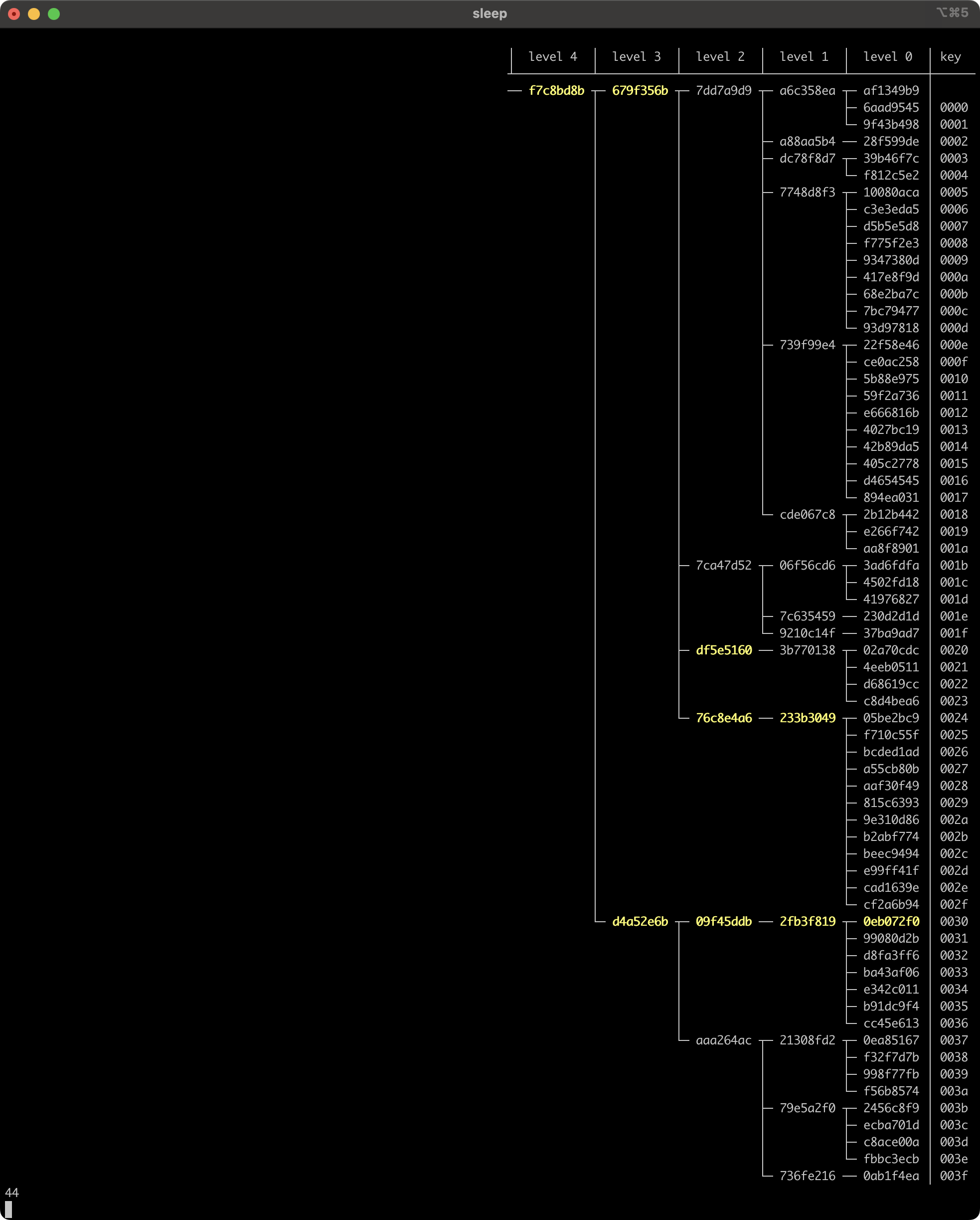
The update to the entry at key 0x0030 caused its parent split, which also caused its grandparent to split. Splits can propagate backwards, but only happen with probability 1/Q.
Quantifying the exact number of expected splits caused by a change is... hard. In a tree with n leaf entries, we expect a path of log_Q(n)+1 nodes from the leaf to the root, of which 1 in Q are boundaries and the other Q-1 in Q aren’t. A split happens when a non-boundary node becomes a boundary, and has conditional probability 1/Q, so we expect at least (log_Q(n)+1) * ((Q-1)/Q) * (1/Q). Splits create new parents that might themselves induce further splits, so the real number is a little more, but we also run out of space when we hit the anchor edge of the tree, so propagation is bounded by that as well. In the end, it’s something on the order of (log_Q(n)+1)/Q.
This still isn’t a complete description of the changes to the tree since we haven’t mentioned merging and the nodes that get deleted during the process. But because we know the tree is pseudo-random and therefore self-balancing, we can infer that on average it must delete the same number of nodes it creates.
There’s a funny kind of symmetry here: only changes to boundary nodes can cause merges, and they’re very likely (1-1/Q) to do so, while only changes to non-boundary nodes can cause splits, and they’re not very likely (1/Q) to do so. But because boundary nodes themselves account for just 1/Q of the nodes overall, it all evens out!
I find it easiest to characterize the process intuitively as “towers are slow to grow and quick to fall”. This is where embracing the skip-list perspective is especially helpful. Nodes at high levels are towers of hashes that all happen to be less than 2^32/Q; every time the hash at the top of a tower changes, it has a small 1/Q chance of growing to the next level (and, if it does, another 1/Q of growing to the level after that, and so on). On the other hand, every time a hash at a lower level of a tower changes, it has a large 1-1/Q chance of pruning the tower right then and there. And even if it happens to survive, it has another 1-1/Q of getting pruned at the next level, and so on.
#Empirical maintenance evaluation
Let’s try it out empirically! Here’s the output of a test that creates a tree (Q = 4 again) with 65,536 entries - one for every key from 0x0000 to 0xffff - and then updates a random entry with a random value 1000 times, recording for each change the height of the tree, total node count, leaf node count, average degree, and number of nodes created, updated, and deleted.
Test [1/3] test.average 1000 random set effects on 65536 entries with Q=4...

initialized 65536 entries in 478ms
updated 1000 random entries in 290ms

           |          avg |    std
---------- | ------------ | ------
height     |        9.945 |  0.898
node count |    87367.875 | 16.784
avg degree |        4.002 |  0.002
created    |        2.278 |  1.977
updated    |       10.006 |  1.019
deleted    |        2.249 |  2.019
Cool! We have an average degree of Q = 4. We expect our total node count to be 65536 + 65536/4 + 65536/4^2 + ... = 65536 * 4/3 = 87381, and it’s pretty close. Here, height is reported as root.level + 1, and we see the same extra unit from the anchor tower scaffolding than the log_4(65536) + 1 = 9 we’d naively expect.
The important parts are the created and deleted numbers. These quantify how robust the tree really is to edits. On average, we update all 10 nodes in the direct path to the root, and additionally create another ~2.28 and delete another ~2.25 along the way. And guess what! (log_4(65536)+1) * (1/4) is exactly 2.25.
But 65,536 entries is still small for a database, and Q = 4 is a toy setting. After all, we only really care about any of this if we’re on a scale where sharing the full state is completely intractable. Let’s try Q = 32 with 2^24 = 16,777,216 entries, where we should expect around (log_32(16777216)+1) * (1/32) = 0.18125 splits and merges per change.
Test [2/3] test.average 1000 random set effects on 16777216 entries with Q=32...

initialized 16777216 entries in 111494ms
updated 1000 random entries in 482ms

           |          avg |    std
---------- | ------------ | ------
height     |        6.548 |  0.517
node count | 17317639.300 |  3.594
avg degree |       32.045 |  0.000
created    |        0.191 |  0.490
updated    |        6.547 |  0.517
deleted    |        0.189 |  0.475
NICE. Making a random change in our key/value store with 16 million entries only requires changing a little less than 7 merkle tree nodes on average.
One final property to highlight: we know for sure that changes within a subtree can never affect the subtrees to its right. Here's the example tree again:
╔════╗
 level 4    ║root║
            ╚════╝
              │
              ▼
            ╔════╗                                                               ┌─────┐
 level 3    ║null║ ─────────────────────────────────────────────────────────────▶│  g  │
            ╚════╝                                                               └─────┘
              │                                                                     │
              ▼                                                                     ▼
            ╔════╗                                                               ╔═════╗                                                     ┌─────┐
 level 2    ║null║ ─────────────────────────────────────────────────────────────▶║  g  ║   ─────────────────────────────────────────────────▶│  m  │
            ╚════╝                                                               ╚═════╝                                                     └─────┘
              │                                                                     │                                                           │
              ▼                                                                     ▼                                                           ▼
            ╔════╗             ┌─────┐   ┌─────┐                                 ╔═════╗             ┌─────┐                                 ╔═════╗
 level 1    ║null║────────────▶│  b  │──▶│  c  │────────────────────────────────▶║  g  ║────────────▶│  i  │────────────────────────────────▶║  m  ║
            ╚════╝             └─────┘   └─────┘                                 ╚═════╝             └─────┘                                 ╚═════╝
              │                   │         │                                       │                   │                                       │
              ▼                   ▼         ▼                                       ▼                   ▼                                       ▼
            ╔════╗   ┌─────┐   ╔═════╗   ╔═════╗   ┌─────┐   ┌─────┐   ┌─────┐   ╔═════╗   ┌─────┐   ╔═════╗   ┌─────┐   ┌─────┐   ┌─────┐   ╔═════╗   ┌─────┐
 level 0    ║null║──▶│a:foo│──▶║b:bar║──▶║c:baz║──▶│d:...│──▶│e:...│──▶│f:...│──▶║g:...║──▶│h:...│──▶║i:...║──▶│j:...│──▶│k:...│──▶│l:...│──▶║m:...║──▶│n:...│
            ╚════╝   └─────┘   ╚═════╝   ╚═════╝   └─────┘   └─────┘   └─────┘   ╚═════╝   └─────┘   ╚═════╝   └─────┘   └─────┘   └─────┘   ╚═════╝   └─────┘
No amount of inserting, updating, or deleting entries before g:... will change the way the entries g:... through m:... organize into the subtree under (3, "g"). This is not a trivial property! It’s only true because our boundary condition is stateless; each node determines its own boundary status independently of its siblings. In particular, if we had used a rolling hash over a window of nodes for determining boundaries at each level, this wouldn’t hold.
#Key/value stores all the way down
All that we have so far is a logical description of a tree structure, and a vague promise that augmenting the logically flat key/value interface with this fancy merkle tree will unlock some interesting syncing capabilities. But how are we actually implementing this?
Key/value stores are typically just B-trees, designed around real-world platform constraints. If we take the task of “merklizing the key/value store” literally and try to pack our tree directly into pages on-disk, we quickly find that there’s inherent conflict between practical B-tree design and the deterministic pseudo-random structure we derived. For example, even though we can set Q to control the average fanout degree, there’s no hard upper limit on how many children a node might end up with, but a basic principle of B-trees is to work strictly inside 4096-byte pages. Maybe we could go back and revise our structure, but then we’re playing a game of tradeoffs, making an already-complicated B-tree even more complicated.
Fortunately, there’s an easier way.
We take an existing key/value store and project the tree structure onto it. This means there are two “key/value stores” in play - an external merklized one, and an internal one used to implement the merkle tree. Every merkle tree node is represented as an internal key/value entry with key [level, ...key] and a value [...hash, ...value?]. Specifically:
- the first byte of every internal key is the
level: u8of the node - the rest of of the internal key
key[1..]is the (external) key of the node’s first leaf entry - the first
Kbytes of the internal value are the node’s hash - leaf nodes store their external value after the hash, in the remaining bytes
value[K..]of the internal value
The most interesting aspect of this mapping is that no parent-to-child or sibling-to-sibling links have to be explicitly represented, since those traversals can be done using the underlying key/value store with the information already present in each node. Given a parent (l, k), we know its first child has internal key [l-1, ...k]. How about sibling iteration? Easy! We iterate over internal entries, breaking when the next internal key has the wrong level byte or when the next entry’s hash (internal value[0..K]) is less than 2^32/Q, since that means it’s the first child of the next parent. Another serendipitous benefit of content-defined chunking!
Decoupling the two trees lets them each do what they do best. Internally, the underlying key/value store can pack whichever entries into whichever pages it wants, with no regard for the merkle-level node boundaries, keeping empty slots for future insertions, and so on. Every update, split, and merge translates directly to a single set or delete of an internal key/value entry. This does mean that the overall asymptotic complexity gets bumped up a logarithmic notch, since every external operation translates into log_Q(n) internal operations.
Implementing the external set/delete operations involves setting or deleting the corresponding leaf node and then propagating up the levels, splitting, merging, or updating the intermediate nodes as needed. There are a few tricky edge cases that make this non-trivial, but our TypeScript and Zig reference implementations are both able to do it in ~500 careful lines of code.
#Applications
So far, we’ve been vague about how these merkle skip lists are useful, casually talking about “syncing” without saying what exactly that means.
We’ll use TypeScript to make things concrete. First, some types for keys and nodes.
type Key = Uint8Array | null

type Node = {
  level: number
  key: Key
  hash: Uint8Array
  value?: Uint8Array // only present if level === 0 && key !== null
}
Syncing will still be directional, where the initiator plays the role of a local client making a series of requests, and the other party plays the role of a remote server responding to those requests. But, to emphasize that the same parties could play either role, we’ll call the server/remote role Source and the client/local role Target.
interface Source {
  getRoot(): Promise<Node>

  getNode(level: number, key: Key): Promise<Node | null>

  getChildren(level: number, key: Key): Promise<Node[]>
}
To be a server, you just need to expose the Source interface methods over an HTTP API, WebSocket connection, or libp2p protocol, etc.
Locally, all we need from the Target tree is the same methods as Source, plus the ability to iterate over a bounded range of merkle nodes at a given level. We’ll also throw the key/value interface methods into there, even though they’re not used by the syncing process itself.
interface Target extends Source {
  nodes(
    level: number,
    lowerBound?: { key: Key; inclusive: boolean } | null,
    upperBound?: { key: Key; inclusive: boolean } | null,
  ): AsyncIterableIterator<Node>

  get(key: Uint8Array): Promise<Uint8Array | null>

  set(key: Uint8Array, value: Uint8Array): Promise<void>

  delete(key: Uint8Array): Promise<void>
}
It’s crucial that this iterator doesn’t break between “parent boundaries” - it’s another place where it’s more appropriate to think of the structure as a skip-list than a tree. In the big example skip-list diagram, nodes(1, { key: "c", inclusive: true }, null) must yield the level-1 nodes with keys c, g, i, and m, even though g was the first child of a different parent.
Cool! Now for the main attraction. Everything that we’ve done so far was all building up to this one function sync.
type Delta = {
  key: Uint8Array
  sourceValue: Uint8Array | null
  targetValue: Uint8Array | null
}

function sync(source: Source, target: Target): AsyncIterable<Delta> {
  // ...
}
sync uses the methods in the Source and Target interfaces to yield Delta objects for every key-wise difference between the source and target leaf entries. This format generalizes the three kinds of differences there can be between key/value stores:
sourceValue !== null && targetValue === nullmeans the source tree has an entry forkeybut the target tree doesn’t.sourceValue === null && targetValue !== nullmeans the target tree has an entry forkeybut the source tree doesn’t.sourceValue !== null && targetValue !== nullmeans the source and target trees have conflicting values forkey.
sourceValue and targetValue are never both null, and they’re never both the same Uint8Array value.
The actual implementation of sync is a depth-first traversal of source that skips common subtrees when it finds them, plus some careful handling of a cursor in the target tree’s range. You can see it in ~200 lines of TypeScript here.
It turns out that this this low-level Delta iterator is an incredibly versatile primitive, with at least three distinct usage patterns.
#Single-source-of-truth replication
Suppose we want to recreate rsync, where Alice is the source of truth and Bob just wants to keep a mirror up-to-date. Bob has his own local tree target and a client connection source to Alice; whenever he wants to update, he initiates a sync and adopts Alice’s version of each delta.
// Bob has a local tree `target: Target` and a
// client connection `source: Source` to Alice

for await (const { key, sourceValue, targetValue } of sync(source, target)) {
  if (sourceValue === null) {
    await target.delete(key)
  } else {
    await target.set(key, sourceValue)
  }
}
It’s that easy! And maybe Bob has other side effects to await for each delta, or additional validation of the values, or whatever. Great! He can do whatever he wants inside the for await loop body; the sync iterator just yields the deltas.
#Grow-only set union
Suppose instead that Alice and Bob are two peers on a mesh network, and they’re both subscribed to the same decentralized PubSub topic, listening for some application-specific events. Bob goes offline for a couple hours, as is his wont, and when he comes back he wants to know what he missed.
In this case, they can both store events in our merklized key/value store using the hash of a canonical serialization of each event as the key. Then when Bob wants to check for missing messages, he initiates a sync with Alice, only paying attention to the entries that Alice has that he doesn’t, and expecting that there won’t be any value conflicts, since keys are hashes of values.
// Bob has a local tree `target: Target` and a
// client connection `source: Source` to Alice
for await (const { key, sourceValue, targetValue } of sync(source, target)) {
  if (sourceValue === null) {
    continue
  } else if (targetValue === null) {
    await target.set(key, sourceValue)
  } else {
    throw new Error("Conflicting values for the same hash")
  }
}
It’s just a minor variation of the last example, but this time it’s not something rsync could help us with. Bob doesn’t want to lose the events the he has that Alice doesn’t, and rsync would overwrite them all. Bob wants to end up with the union of his and Alice's events, so he needs to use our async delta iterator. And when he's done, Alice can flip it around and initiate the same kind of sync with Bob to check for events she might have missed!
Today, one standard approach to this problem is to use version vectors (not to be confused with vector clocks), but that requires events to have a user ID, requires each user to persist their own version number, and produces vectors linear in the total number of users to ever participate. In many systems, this is fine and even natural, but it can be awkward in others that have lots of transient users or are supposed to be anonymous. Why couple retrieval with attribution if you don’t have to? Merkle sync lets us achieve the same thing while treating the events themselves as completely opaque blobs.

(And what if retrieving a specific event fails? If Eve skips a version number, does Bob keep asking people for it until the end of time?)
#Merging state-based CRDT values
It’s cool that merkle sync can implement grow-only sets and single-source-of-truth replication, and they’re real-world use cases, but neither are “peer-to-peer databases” in a true sense. What if we want multi-writer and mutability?
Merkle sync doesn’t magically get us all the way there, but it brings us close. You can use it to merge concurrent versions of two databases, but you need your own way to resolve conflicts between values.
// `merge` is an application-specific value resolver,
// e.g. parsing structure out of the values and using
// a causal order to choose and return a winner.
declare function merge(key: Uint8Array, sourceValue: Uint8Array, targetValue: Uint8Array): Uint8Array

for await (const { key, sourceValue, targetValue } of sync(source, target)) {
  if (sourceValue === null) {
    continue
  } else if (targetValue === null) {
    await target.set(key, sourceValue)
  } else {
    await target.set(key, merge(key, sourceValue, targetValue))
  }
}
As you might expect, the merge function must be commutative, associative, and idempotent in order to be well-behaved.
- commutativity:
merge(k, a, b) == merge(k, b, a)for allk,a, andb - associativity:
merge(k, a, merge(k, b, c)) == merge(k, merge(k, a, b), c)for allk,a,b, andc - idempotence:
merge(k, a, a) == afor allkanda(although this is more of a conceptual requirement sincemergewill never be invoked with identical values)
To get multi-writer mutability, Alice and Bob wrap their values with some tag that lets them compute a deterministic causal ordering. Here’s a naive implementation of merge that uses last-write-wins timestamps.
type Value = { updatedAt: number; value: any }

function merge(key: Uint8Array, sourceValue: Uint8Array, targetValue: Uint8Array): Uint8Array {
  const decoder = new TextDecoder()
  const s = JSON.parse(decoder.decode(sourceValue)) as Value
  const t = JSON.parse(decoder.decode(targetValue)) as Value
  if (s.updatedAt < t.updatedAt) {
    return targetValue
  } else if (t.updatedAt < s.updatedAt) {
    return sourceValue
  } else {
    return lessThan(sourceValue, targetValue) ? sourceValue : targetValue
  }
}

// used to break ties for values with the same timestamp
function lessThan(a: Uint8Array, b: Uint8Array): boolean {
  let x = a.length
  let y = b.length

  for (let i = 0, len = Math.min(x, y); i < len; i++) {
    if (a[i] !== b[i]) {
      x = a[i]
      y = b[i]
      break
    }
  }

  return x < y
}
Now, when Alice and Bob sync with each other, they end up with the most recent values for every entry. If they want to “delete” entries, they have to settle for leaving tombstone values in the key/value store that are interpreted as deleted by the application, but this is common in distributed systems. Also note that merge doesn’t have to return one of sourceValue or targetValue - for some applications there could be a merge function that actually combines them in some way, as long as it’s still commutative and associative - but arbitrating between the two is probably the most common case.
What we’ve essentially implemented is a toy state-based CRDT, which is a whole field of its own. Similar to the grow-only set example, the utility of merkle sync here is not that it provides a magic solution to causality, but rather that it enables a cleaner separation of concerns between layers of a distributed system. Alice and Bob can use whatever approach to merging values that makes sense for their application without worrying about the reliability of decentralized PubSub delivery or having to track version vectors for retrieval.
#Concurrency constraints
You might be worried about operating on the target tree mid-sync. Operations can cause splits and merges at any level - will this interfere with the ongoing depth-first traversal? Fortunately, this is actually fine, specifically due to the property that mutations in any subtree never affect the subtrees to their right. The target tree can always safely create, update, or delete entries for the current delta’s key.
Unfortunately, the same can’t be said for the source tree. The source needs to present a fixed snapshot to the target throughout the course of a single sync, since the intermediate nodes are liable to disappear after any mutation. This means syncing needs to happen inside of some kind of explicit session so that the source can acquire and release the appropriate locks or open and close a read-only snapshot.
#Implementations
The animations and tests we saw in previous sections were run on a reference implementation called Okra. Okra is written in Zig, using LMDB as the underlying key/value store.
As a wrapper around LMDB, Okra has fully ACID transactions with get(key), set(key, value), and delete(key) methods, plus a read-only iterator interface that you can use to move around the merkle tree and access hashes of the merkle nodes. Only one read-write transaction can be open at a time, but any number of read-only transactions can be opened at any time and held open for as long as necessary at the expense of temporarily increased size on-disk (LMDB is copy-on-write and will only re-use stale blocks after all transactions referencing them are closed). The Zig implementation does not implement sync, since syncing is async and so closely tied to choice of network transport.
Okra also has a CLI, which can be built with zig build cli after installing Zig and fetching the submodules. The CLI is most useful for visualizing the state of the merkle tree, but can also be used for getting, setting, and deleting entries.
There is also a JavaScript monorepo at canvasxyz/okra-js with native NodeJS bindings for the Zig version, plus a separate abstract pure-JavaScript implementation with IndexedDB and in-memory backends.
#Conclusions
I’ll step into the first person for a friendly conclusion. I started looking into merklized databases last summer in search of a reliable persistence layer to complement libp2p’s GossipSub, and found that variants of deterministic pseudo-random merkle trees were an active early research area. I was ecstatic.
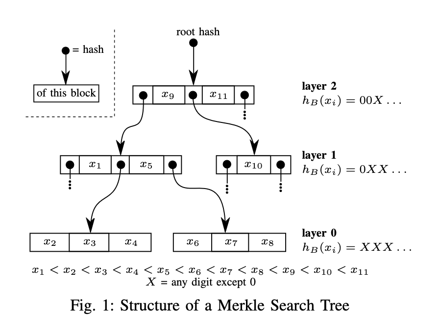
The original paper on Merkle Search Trees (MSTs) describes something very different than the approach I ended up pursuing. MSTs are more like classical B-Trees where the intermediate nodes store values too: each key/value entry’s hash determines its level in the tree, and nodes interleave values with pointers to nodes at the level below. It’s actually quite complicated.
Prolly Tree seems to be the consensus name for the bottom-up/dynamic chunking approach. I first saw the idea described in this blog post, but it appears to have originated in the now-dead project attic-labs/noms. Dolt, a relational database with git-like characteristics, has a great blog post about Prolly Trees that spends a lot of time focusing on ways to tune the chunk size distribution. Our naive u32(node.hash[0..4]) < 2^32/Q condition gives us parents with Q children on average, but in a geometric distribution with more smaller chunks than bigger chunks. Dolt took on the challenge of implementing a native Prolly Tree directly on-disk, so they reworked the chunk boundary condition to get chunks to fit more consistently into 4096-byte pages, transforming the distribution on the left into the distribution on the right.
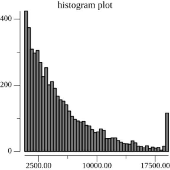
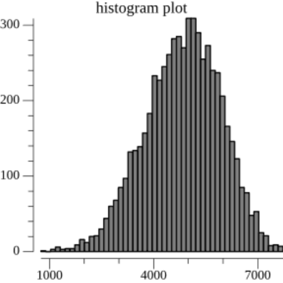
A simple solution is to use the size of the current chunk as an input into the chunking function. The intuition is simple: if the probability of chunk boundary increases with the size of the current chunk, we will reduce the occurrence of both very-small and very-large chunks.
This was something I planned to do, but shelved as the prospect of working on top of existing key/value stores came into focus. As far as I can tell, Okra’s generic key/value backend is a novel approach, and hinges on the specific way the fixed anchors give nodes stable (level, key) identifiers. Or maybe just rotating the tree 45 degrees, I can't really tell.
I don’t know enough about either database internals or distributed systems to thoroughly compare the trade-offs between the Okra way and a full-fledged on-disk Prolly Tree. I’m really happy with how easy Okra was to implement, especially in the browser context over a single IndexedDB object store, and personally place a high value on that kind of simplicity as long as it meets my needs. But I also know that lots of serious engineering went into Dolt and would bet it performs better at scale. Another major aspect of Dolt’s implementation is that it has git-like time-travel. Like LMDB, Dolt is copy-on-write, but it keeps the old blocks around so that it can access any historical snapshot by root hash.
One future direction that I’m excited to explore is packaging Okra as a SQLite plugin. I think it could work as a custom index that you can add to any table to make it “syncable”, in any of the three replicate/union/merge usage patterns, with another instance of the table in anyone else’s database.
More generally, I find myself constantly impressed by the unreasonable utility of merklizing things. As always, the friction is around mutability and identity, but pushing through those headwinds seems to consistently deliver serendipitous benefits beyond the initial goals. We’re used to thinking of “content-addressing” as an overly fancy way of saying “I hashed a file” (or at least I was), but I’m coming around to seeing a much deeper design principle that we can integrate into the lowest levels of the stack.
Overall it seems like there's an emerging vision of a lower-level type of decentralization, where the data structures themselves sync directly with each other. The modern computer has hundreds of databases for various kinds of apps at all times - what if the application layer didn’t have to mediate sync and replication logic at all? What if you could make a social app without writing a single line of networking code?
Many thanks to Colin McDonnell, Ian Reynolds, Lily Jordan, Kevin Kwok, and Raymond Zhong for their help in editing.